Robot Foosball Part 3: Artificial Intelligence

February 22, 2014

Introduction

This is the AI part of my foosball project. Be sure to check out part 1 and part 2!

From my (basic) understanding of machine learning there’s the following:

Supervised Learning - Given some labeled data, learn a general function to determine the labels for that data without over-fitting. E.g. Classification and Regression
Unsupervised Learning - Given some unlabeled data, find structure in the data. E.g. Clustering and Baum-Welch
Reinforcement Learning - Given some environment, perform actions to observe the consequences. Use these experiences to learn the appropriate actions to maximize expected reward. E.g. Q-Learning and Policy Search

The project was my chance to dabble in a real-world application of Reinforcement Learning. I will start by introducing some of the basic ideas behind Reinforcement Learning before talking about my experience in applying it to my foosball robot. The majority of this information is available through Edx’s course on artificial intelligencee, a class I had the privilege of taking in person while I was a student a UC Berkeley. If you find this post interesting, you will do yourself more justice taking the online class since this post almost serves as my own personal cliff notes of one small section of the class. Remember all the code is available on my github.

Markov decision process

I find it fascinating that we can program an agent to learn by experiencing the consequences of its actions in a given environment. Such environments are often modeled by a Markov decision process which is defined by the following:

$\begin{align} \text{1. } & \normalsize S \small \text{, a set of states} \\ \text{2. } & \normalsize A \small \text{, a set of actions} \\ \text{3. } & \normalsize P_{a}(s,s')=Pr(s'|s,a) \small \text{, state transition probabilities for a given state and action } \\ \text{4. } & \normalsize R_{a}(s,s') \small \text{, rewards for state transitions for a given state and action } \\ \end{align}$

The image above from Wikipedia portrays an example of an MDP. MDPs allow us to represent decision problems (what action do I take?) given uncertainty (the nature of our world). It also simplifies things (mostly the math) by allowing us to assume the next state only depends on the current state and action, and not any previous states or actions. With MDPs, we generally want to find a policy. A policy returns an action for every given state. The goal is to find a policy that maximizes expected utility (basically the rewards), this is the optimal policy. I will talk about different ways to determine an optimal policy before introducing Q-learning.

Model Based Learning

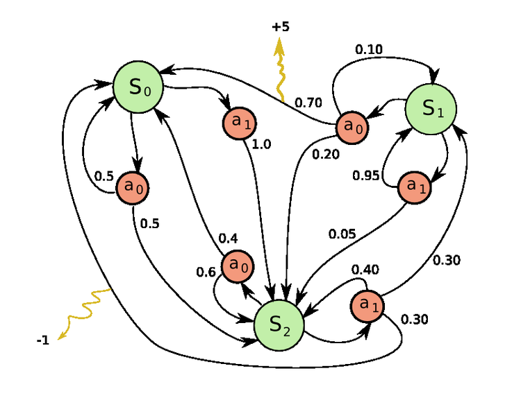
As you can see in the diagram above, taking an action from a green colored state results in an orange colored “probabilistic state” where the outcome is nondeterministic. There’s a 70% chance that taking action a_0 from state S_1 will result in a +5 reward and end in state S_0, a 20% chance you will end up in state S_2, and a 10% chance that nothing will change. These orange-states are call Q-states and in order for us to write algorithms using MDPs we need to be able to quantify their values. If we think about it intuitively, what would be the value of action a_0 from state S_1? Well, we know there’s a 70% chance of getting a reward of 5, etc…How about .70(value of state S_0 + 5 reward) + .20(value of state S_2) + .10(value of state S_0)? The value of a Q-state (Q-value) can be defined as the weighted sum over all possible transition states of the rewards plus future (discounted) values of the new state, where the weights are the probabilities of each transition:

$\begin{align} & Q^{*}(s,a) = \sum_{s'} P_{a}(s,s')[R_{a}(s,s') + \gamma V^{*}(s')] \\ \end{align}$

The optimal value of a state (a regular, green state) is therefore the maximum of the Q-values. Basically the value of a state is the best action because Q-values represent state-action pairs:

$\begin{align} & V^{*}(s) = max_{a} Q(s,a) \\ & V^{*}(s) = max_{a} \sum_{s'} P_{a}(s,s')[R_{a}(s,s') + \gamma V^{*}(s')] \\ \end{align}$

Note: Gamma in these equations can represent greediness. If gamma is 0 the Q-value becomes a weighted sum of the rewards. In our example the Q_value(S_1, a_0) would just be .70(5 reward) if gamma was 0. That means we don’t care if an action gets us killed, as long as we get the largest instantaneous reward between all the other actions. Alternatively, the higher gamma is, the more we consider our future prospects. I keep gamma at .99 for this project.

Now that we can quantify states and actions, we can run an algorithm called Value Iteration to determine the optimal state values:

$\begin{align} \text{1. } & \forall s\in\normalsize S \small \text{ Set } V_{0}(s) = 0 \\ \text{2. } & \text{Update } V_{k+1}(s) \leftarrow max_{a}\sum_{s'} P_{a}(s,s')[R_{a}(s,s') + \gamma V_{k}(s')] \\ \text{3. } & \text{Repeat until convergence} \\ \end{align}$

Value Iteration allows us to determine optimal values as well as the optimal policy for a given state. However, in order to determine the best action given the value of a state, we have to do a bit of work. Calculating the actions from values is called policy extraction and requires you to use the known optimal values, transition probabilities, and rewards to compute the best action. Remember a policy, is just a mapping of states to actions, a table we can use to determine what actions to take given a state.

$\begin{align} & \pi^{*}(s) = argmax_{a} \sum_{s'} P_{a}(s,s')[R_{a}(s,s') + \gamma V^{*}(s')] \\ \end{align}$

As you can see, determining the optimal policy given state values still requires some work. Another algorithm that could converge faster to the optimal policy is called Policy Iteration:

$\begin{align} \text{1. } & \text{Start with some policy } \pi \text{ and run policy evaluation until the values converge} \\ \text{2. } & \text{Extract a new policy from those values with policy extraction} \\ \text{3. } & \text{Repeat until the policy converges} \\ \end{align}$

Policy Evaluation is similar to Value Iteration, except you do not take a max over the available actions because you are limited to your policy:

$\begin{align} \text{1. } & \forall s\in\normalsize S \small \text{ Set } V^{\pi}_{0}(s) = 0 \\ \text{2. } & \text{Update } V^{\pi}_{k+1}(s) \leftarrow \sum_{s'} P_{\pi(s)}(s,s')[R_{\pi(s)}(s,s') + \gamma V^{\pi}_{k}(s')] \\ \text{3. } & \text{Repeat until convergence} \\ \end{align}$

The idea here is to pick some policy. Using the diagram above, let’s say we pick a policy of “always takes actions a_0”. Run Policy Evaluation to determine how good that policy was. Now that we’ve gained some information from the environment, we can extract a better policy and repeat. So we have two algorithms we can use to determine the optimal policy, Value Iteration and Policy Iteration.

Model Free Learning

Value Iteration and Policy Iteration are great for when you know the all the parameters to your MDP, but what if you don’t? If I apply Value Iteration to foosball, I would have to know all the possible resulting states from hitting the ball in position (200, 100) with my player in position (210, 100), as well as the probabilities for each state. Then I’d need to know this for every possible player-position/ball-position/action combination. And remember, my gamestate is a discretized version of the real world. If my ball is in position (200,100) there’s probably a millimeter or three of real-world tolerance and a whole host of different angles the player could strike the ball with. This would be very difficult to model.

In the general case, it is certainly possible to learn those parameters through machine learning but spending the time learning the parameters seems wasted when that only gets you half way there (you still have to run policy or value iteration).

Fortunately there is a better way! Instead of learning the parameters of the MDP we could try estimating the state values by sampling actions in the actual environment; take an action according to some policy, experience the instantaneous reward, and use that to update your estimate of the state value. This is called temporal difference learning.

$\begin{align} & V^{\pi}_{sample}(s) = R_{\pi(s)}(s,s') + \gamma V^{\pi}_{estimate}(s')\\ & V^{\pi}_{estimate}(s) \leftarrow (1-\alpha)V_{estimate}^{\pi}(s) + (\alpha)V^{\pi}_{sample}(s) \\ \end{align}$

Alpha is the learning rate, it determines how fast you learn, or how much weight you want to give new experiences. What we’re doing here is calculating a running exponential average for the state value. Overtime this will eventually converge to the correct values for that policy. So now, all we have to do is use policy extraction on our newly estimated state values to improve our policy and repeat until the policy converges. This would essentially be policy iteration where we use estimates for the state values. There’s one problem:

$\begin{align} & \pi_{new}(s) = argmax_{a} \sum_{s'} P_{a}(s,s')[R_{a}(s,s') + \gamma V_{estimate}(s')] \\ \end{align}$

Remember policy extraction takes a bit of work and it requires us to know the reward and state transition probabilities for the MDP. We’ve taken a model-free approach to learning the state values (for a policy), but we can’t use this knowledge to improve our policy! We can’t use policy extraction unless we also sample transition probabilities and rewards, but we had just decided that was a waste of time…

Let’s go back to the drawing board. Why did we want state values in the first place? Because we’re trying to find the optimal policy. If you look at the equation for policy extraction, it doesn’t really seem to fit well with state values. It almost seems to fit better with…. Q-values! Wait a second…look at the first equation where I define the Q-value for a state.

$\begin{align} & \pi^{*}(s) = argmax_{a} \sum_{s'} P_{a}(s,s')[R_{a}(s,s') + \gamma V^{*}(s')] = argmax_{a} Q^{*}(s,a) \\ \end{align}$

Policies are just the best action from a given state and Q-values represent actions! So policies should really be extracted from Q-values not state values. What if we learn the Q-values through sampling instead of the state values? What would the sample look like? Well since the value of a state is just the max of the Q-values, it’s no surprise that they are very similar.

$\begin{align} & Q_{sample}(s,a) = R_{a}(s,s') + \gamma max_{a'}Q_{estimate}(s',a') \\ & Q_{estimate}(s,a) \leftarrow (1-\alpha)Q_{estimate}(s,a) + (\alpha)Q_{sample}(s,a) \\ \end{align}$

This is Q-learning and this time we get control over which actions to take, where-as with estimated state-values we were limited to a fixed policy (that we couldn’t improve). Q-learning is awesome because it will converge to the optimal Q-values (and therefore policy). Except you have to make sure you explore enough (state and actions) and remember to lower the learning rate (alpha) over time. Since Q-learning will converge to optimal values, it just becomes a question of how fast can I converge which is really a question of exploration vs exploitation (how do I chose which actions to take). That problem can be solved many ways, a simple solution is to take a random action with some probability, epsilon, or otherwise take the best action according to your Q-values. You can also start with some high value for epsilon and decrease it over time. Here’s the basic algorithm for Q-learning:

$\begin{align} \text{1. } & \forall s\in\normalsize S \small \text{ and } a\in\normalsize A \small \text{ set } Q_{estimate}(s,a) = 0 \\ \text{2. } & \text{Take action a from state s} \\ \text{3. } & \text{Recive reward as you transition to a new state, s'} \\ \text{4. } & \text{Update } Q_{estimate}(s,a) \text{ with } Q_{sample}(s,a) \\ \text{5. } & \text{Repeat 2-4 until convergence} \\ \end{align}$

There’s still one problem (I promise this is the last one)! Consider the two foosball states below:

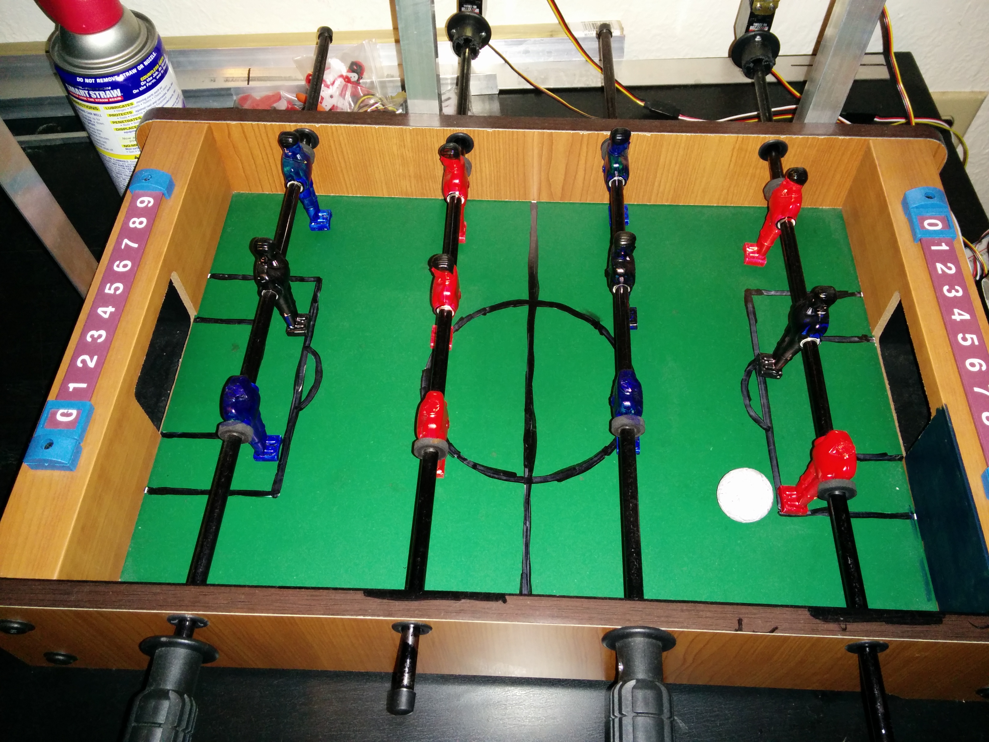
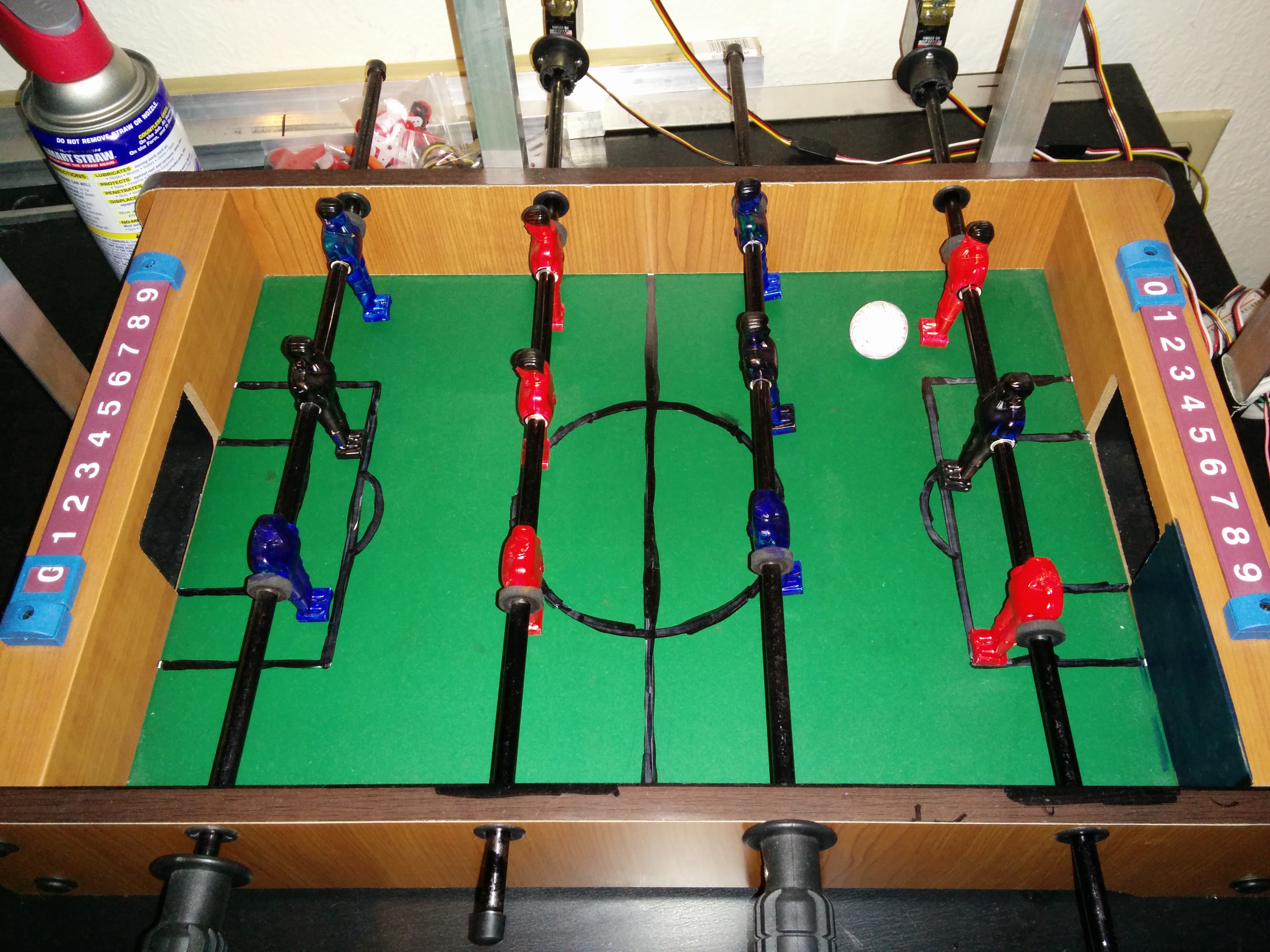
In both cases the agent should probably hit the ball right? Let’s assume the first image is a state we’ve already visited many times and know the best course of action is to hit the ball. The second image however is entirely new and the agent has no idea what to do. The problem here is that we have no way of transferring experiences between similar states. We have to visit every state-action pair combination to learn the optimal values and in foosball that would be:

$\begin{align} & (320*240 \text{ball positions})(40 \text{player y-positions})^{(4 \text{rows})}(5 \text{player angles})^{(4 \text{rows})} \end{align}$

That’s 122 trillion states and that doesn’t even include Q-states. Ain’t nobody got time OR space for that. It would take forever to visit all those states and we probably don’t have enough memory to store all of the Q-values. There must be a better way!

The idea is to mathematically represent states as a linear combination of weights and features, that way we can generalize and transfer experiences between similar states. Features are meant to describe certain characteristics of a state, or in our case, a Q-state, which means we are describing state-action pairs. One feature can represent the possibility of hitting the ball, another feature can represent the possibility of allowing the enemy to score a goal. As the agent learns it adjusts the weights associated with each feature. For example, if the enemy were to score on the agent (which results in a negative reward) while the second feature I mentioned was active, then we would lower the weight for that feature based on the difference between the estimated value for the Q-state and actual (negative) reward we had just received. This is called approximate Q-learning and the algorithm is as follows:

$\begin{align} \text{0. } & \text{Define } Q(s,a) = w_{i}f_{1}(s,a) + w_{2}f_{2}(s,a) + w_{n}f_{n}(s,a) \\ \text{1. } & \forall w\in\normalsize W \small \text{ set } w_{i} = 1 \\ \text{2. } & \text{Take action a from state s} \\ \text{3. } & \text{Recive reward as you transition to a new state, s'} \\ \text{4. } & \text{Update weights } w_{i} \leftarrow w_{i} + \alpha(correction)f_{i}(s,a) \\ \text{5. } & \text{Repeat as needed} \\ \end{align}$ $\begin{align} correction = (R_{a}(s,s') + \gamma max_{a'}Q(s',a')) - Q(s,a) \end{align}$

When you update the weights in step 4, you are essentially “correcting” them. The correction is the difference between what we thought the Q-value was for the action we took with the actual reward we received plus the best possible (discounted) Q-value for the new state. Those two numbers should be fairly close. You will also notice that we down-weight the correction by alpha, our learning rate and upscale the correction by the actual feature value. The larger (or more prominent) a feature is, the larger it is rewarded for doing good and harsher it is punished for doing bad.

#Implementation

Implementing approximate Q-learning in my foosball robot turned out to be more difficult than I anticipated. I spent days tweaking the rewards, playing around with many different features, until I was able to get the agent to learn something worth showing. The performAction method runs (more or less) every time the vision algorithm updates the gameState if agent is not still doing its thing.

public class ApproximateQLearningAgent extends AbstractFoosballAgent {
  //Weights initialized to 1
  private List<Float> featureWeights = new ArrayList<Float>(Arrays.asList(new Float[] { 1f, 1f, 1f, 1f }));
    
  // Learning Rate
  private float alpha = .3f;
    
  // Percent Chance for Random Action
  private float epsilon = .1f;
    
  // Discount Factor
  private float gamma = .99f;
  
  public void performAction() {
    this.updateWeights();
    // Take Action if no one has scored
    if (gameState.getPlayerThatScored() == null)
      this.takeAction();
    else {
      this.resetRound();
    }
  }

  public void takeAction() {
    if(Math.random() < epsilon) {
      this.takeRandomAction();
    } else {
      this.takeBestAction();
    }
  }

}

The update weights method is shown below. At this point we are in state s’ and will receive our reward from the previous action. To update the weights, we find the best possible Q-value by iterating over every possible action, and calculating the Q-value with those actions, the current state, and feature weights.

Note: while there are approximately 80 discrete y-positions the bottom player can be in, I’ve reduced this to 40 because there are only 40 possible servo angles and it will significantly cut down the number of possible actions I need to iterate through.

private void updateWeights() {
  //Find the maxQValue by calculating the QValue for every action from this state
  float maxQVal = -Float.MAX_VALUE;
  // Max over all possible actions (~40,000)
  for (int rowOneYPos = 0; rowOneYPos < 40; rowOneYPos++) {
      for (int rowThreeYPos = 0; rowThreeYPos < 40; rowThreeYPos++) {
          for (PlayerAngle rowOneAngle : PlayerAngle.getValues()) {
              for (PlayerAngle rowThreeAngle : PlayerAngle.getValues()) {
                  float qVal = 0;
                  List<Float> featureVals = this.getFeatureValuesCurrentStateAndActions(rowOneYPos, rowThreeYPos, rowOneAngle, rowThreeAngle);
                  for (int i = 0; i < featureVals.size(); i++) {
                      qVal += featureWeights.get(i) * featureVals.get(i);
                  }
                  if (qVal > maxQVal) {
                      maxQVal = qVal;
                  }
              }
          }
      }
  }
  float diff = this.getReward() + gamma * maxQVal - prevQVal;
  System.out.println("UPDATE WEIGHTS diff=" + diff + "\tbestQVal=" + maxQVal + "\tprevQ" + prevQVal + "\tprevFeatures=" + prevFeatureVals);
  for (int i = 0; i < featureWeights.size(); i++) {
      featureWeights.set(i, featureWeights.get(i) + alpha * diff * prevFeatureVals.get(i));
  }
  System.out.println("UPDATE WEIGHTS New Weights=" + featureWeights);
}

Before I talk about the specific rewards and features used in the demo video I wanted to give some practical advice I learned while getting this to work. The first two are the most important:

When you take a non-random action make sure you randomly pick between all actions that had the highest Q-value
Keep your feature values between [0,1] otherwise the update step will cause wild fluctuations in weights. Mine are binary. Put another way, normalize your features.
Remember that feature values are supposed to characterize state-action pairs (repeat this to yourself)
Instantaneous rewards are very important for learning, do not rely on end-state rewards (such as goals)
Your agent will not perform actions that are not featured/rewarded
Start with 1 feature/reward before adding more (baby steps!)

I reward the agent for keeping players in line with the ball, for blocking incoming balls, and also hitting the ball forward. Of course there are rewards for scoring a goal (and a negative reward for getting scored on) but those rewards are much less vital to the learning process, at least in my case. The features reflect the rewards; they characterize actions that could potentially block an incoming ball, hit the ball forward if it is within reach, and also try to move the ball in the y-axis if it is directly behind and within reach. As a result those are the only things this agent does.

Demo

This video below shows some training matches. It is certainly far from perfect, since there are so many actions available to the agent, it can take up to 1 second to calculate the 40,000 Q-values (twice), so I have to hit the ball slow. I wish I had a more powerful computer :)

Conclusions

My goal with this project was to implement reinforcement learning in a physical environment and get it to work reasonably well. Physical environments are lot harder than simulations due to noise and uncertainty. Nonetheless, I think I’ve accomplished my goal and I have certainly learned a lot. However, the project is not without pitfalls. The agent certainly behaves as expected, but not without noticeable issues, a lot of which can be traced back to noise. Also the large action-space makes it difficult to calculate the next action quickly enough, but a faster computer would easily fix this. If I spend more time improving all aspects of this project (better foosball table, vision algorithm, faster computer, noise reduction), I can probably get the robot to always block an incoming ball, hit the ball forward, etc. But that’s not necessarily how you play foosball, and what happens if the ball gets stuck in the corner (like it did in the video)? Of course I can improve my features, notice how none of my features even consider the enemy position, but I can only go so far with additional features. This is where my model starts to shows its weakness. In foosball, actions are much more complex than just “angle players forward”. Real actions in foosball, are a string of actions in my model. For example, the action “slide the ball over then hit it” or “bounce the ball back and forth then ricochet it off the wall” is what people normally do. If someone was trying to build a truly amazing foosball robot, they would most likely be better off using some physics simulations or treating the game as turn-based game where the offense has a plethora of complex actions to chose from, while the defense just has to block the ball. Maybe you can use Q-learning to train those complex actions! :)